This tutorial describes how to build a QSPR model using Alvascience tools. The selected endpoint is the aqueous solubility (LogS). The scope of this tutorial is not to propose new models for aqueous solubility but to describe, step-by-step, the development of QSAR/QSPR regression models, from data curation to the use of models with a new set of molecules.
This tutorial consists of four steps:
- Data curation (alvaMolecule)
- Molecular descriptors calculation (alvaDesc)
- Models development (alvaModel)
- Model application and test (alvaRunner)
1. Data curation (alvaMolecule)
The dataset used in this tutorial is described in Sorkun, M. C., Khetan, A., & Er, S. (2019). AqSolDB, a curated reference set of aqueous solubility and 2D descriptors for a diverse set of compounds. Scientific Data, 6(1), 143. https://doi.org/10.1038/s41597-019-0151-1 and includes 9982 chemicals with experimental values of aqueous solubility. AqSolDB is publicly available and can be downloaded from Harvard Dataverse Repository.
The downloaded file (curated-solubility-dataset.tab) is a tabbed text file containing the molecule representations (ID, SMILES, InChi...), the experimental aqueous solubility (Solubility) expressed as LogS and a few calculated 2D descriptors. 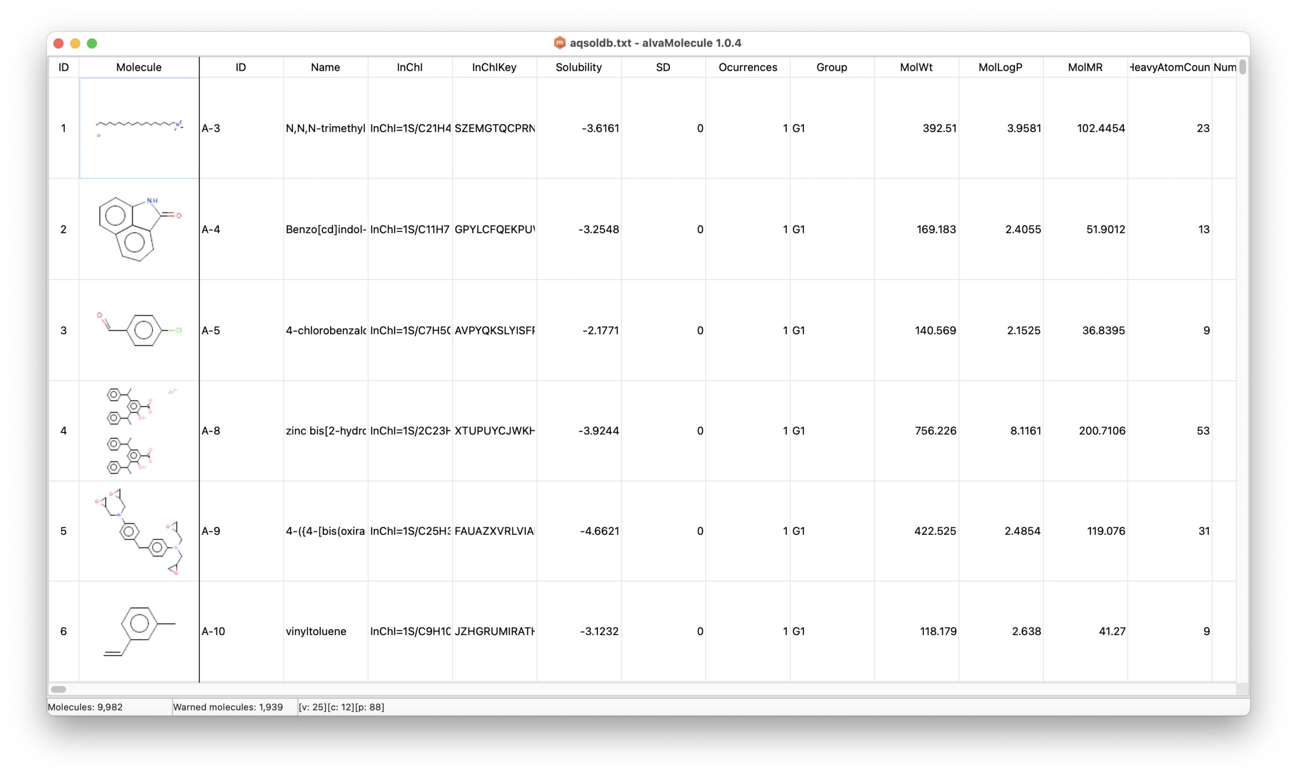
alvaMolecule can load tabbed text files with headers if the first column is the SMILES column. The curated-solubility-dataset.tab has therefore been modified to have the SMILES representation in the first column.
Once prepared, the dataset has been loaded in alvaMolecule.
The first step has been to represent the whole dataset in the aromatic form using the menu Structures –> Aromaticity –> Aromatic form. This operation has been performed in order to avoid the identification of erroneous aromaticity during the check of the structures. This is an important step considering that different cheminformatics tools can use different aromatic representations.
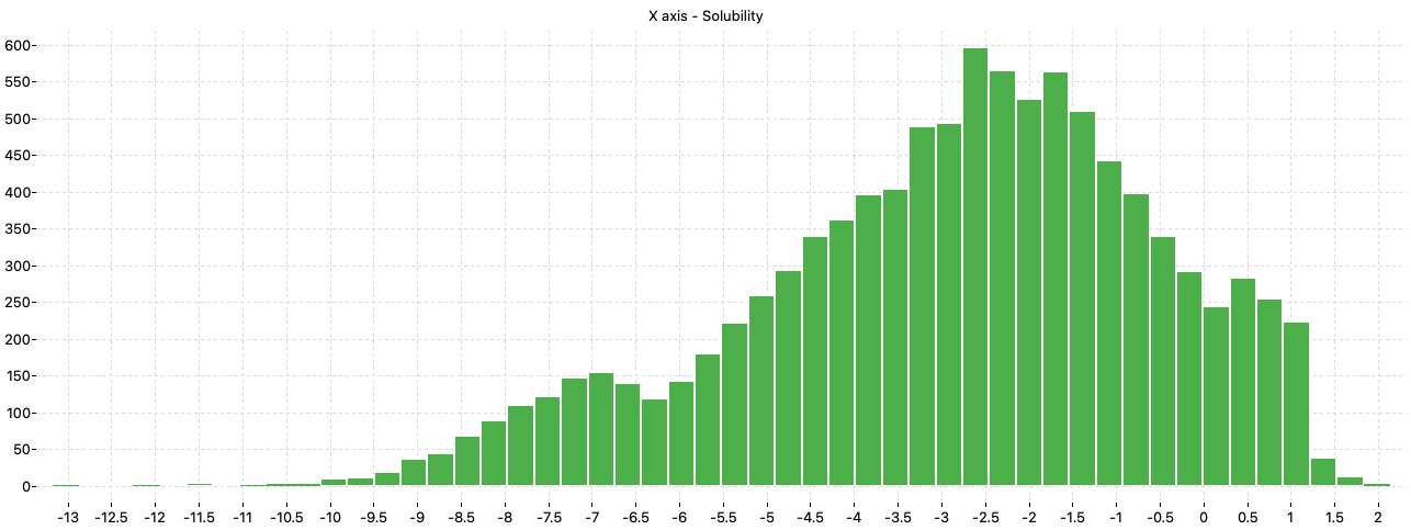
A preliminary analysis of the distribution of the solubility values shows that the majority of the compounds have solubility values in the range between –9 and 1.5 while few chemicals have values lower than –9 or higher than 1.5.
The next step is the calculation of the molecular descriptors (Tools –> Calculate properties).
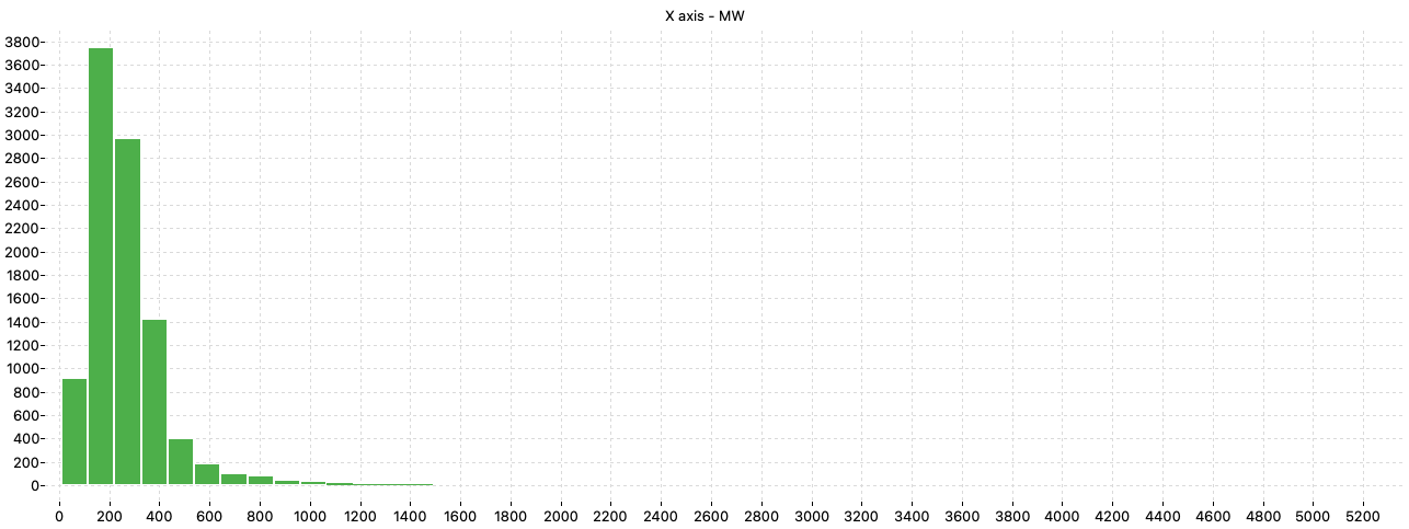
The analysis of the distribution of the molecular weight (MW) in the dataset shows that the majority of the molecules have MW lower than 800 but there are molecules having MW greater than 2000.
Since aqueous solubility is generally related to octanol-water partition coefficient, the ALOGP descriptor was also checked.
ALOGP (Ghose, A. K., Viswanadhan, V. N., & Wendoloski, J. J. (1998). Prediction of hydrophobic (lipophilic) properties of small organic molecules using fragmental methods: An analysis of ALOGP and CLOGP methods. Journal of Physical Chemistry A, 102(21), 3762–3772. https://doi.org/10.1021/jp980230o) is a LogP additive model based on fragment contributions and cannot be calculated for molecules having fragments not included in the original paper. ALOGP cannot be calculated for 1037 molecules of the considered dataset.
The final step is the structure checking (Tools –> Check structures).
The structure checking highlights the presence of 33 molecules with unusual valences and 1098 molecules with multiple structures (i.e. salts, ionic liquids..). The molecules with unusual valences in this dataset are usually radical molecules.
Molecules with unusual valences and for which it was not possible to calculate the ALOGP were excluded for the subsequent analysis.
The resulting dataset including 8826 molecules was saved by alvaMolecule to be imported in alvaDesc.
2. Molecular descriptors calculation (alvaDesc)
The file prepared using alvaMolecule has been loaded in alvaDesc to calculate the molecular descriptors that will be used for the model development.
Using alvaDesc all 2D descriptors has been calculated, for a total of 4179 descriptors.
The distribution of the molecular weight for the 8826 molecules saved by alvaMolecule is better than before, but there are still a few molecules having high molecular weight.
Some preliminary analysis can be performed using alvaDesc, such as t-SNE and principal component analysis (PCA).
The t-SNE analysis performed using all the descriptors shows the presence of different clusters of similar molecules, but in this case does not provide any evident insights.
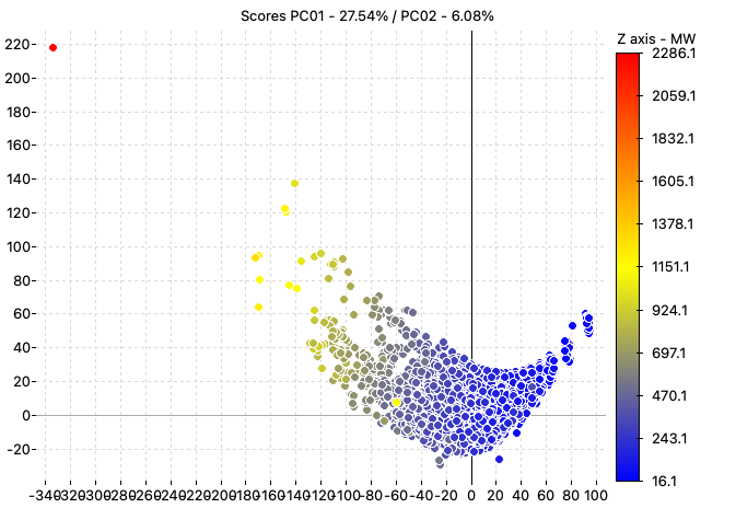
The PCA analysis performed using all the calculated descriptors highlights the presence of an outlier in the dataset, the molecule ID A-2512 (the red point in the chart).
The whole dataset including the calculated descriptors and the experimental values (imported as external variables) was exported as an alvaDesc project.
3. Models development (alvaModel)
The alvaDesc project has been imported in alvaModel.
Two different master dataset have been prepared using alvaModel:
- Master_A: including all molecules except the outlier (molecule ID A-2512). This dataset comprises 8825 molecules.
- Master_B: including all molecules having nStructures = 1 and MW < 850. This dataset comprises 8731 molecules.
Both datasets were split into a training set that includes 60% of the molecules and a test set containing the remaining 40% of the molecules using venetian blinds.
The baseline model used in this tutorial is the ESOL, Estimated SOLubility (logS) for aqueous solubility (Delaney, J. S. (2004). ESOL: Estimating aqueous solubility directly from molecular structure. Journal of Chemical Information and Computer Sciences, 44(3), 1000–1005. https://doi.org/10.1021/ci034243x) included in alvaDesc.
ESOL model calculated by alvaDesc is defined as:
![]()
ESOL model has an R2 = 0.703 when calculated on the Master_A dataset.
The alvaModel Automatic models generation allows to identify the best models using genetic algorithms. Since the genetic algorithms could find local optimum, the solubility models have been searched by running Automatic models generation several times.
All calculated descriptors have been selected for automatic models generation, excepts the ESOL descriptor, Drug-like indices and the external variables included the original AqSolDB dataset. Before launching the genetic algorithms, all constant and near-constant descriptors have been removed from the dataset.
Automatic models generation has been run using the following options:
- Population size: 30
- Maximum number of iterations: 10,000
- Maximum number of features: 5
- Score: Q2 5-fold (venetian blinds)
- Model type: ordinary least squares (OLS)
Several models have been found, most of them include a LogP-based descriptor. The best models include the LOGPcons descriptor (consensus model based on 3 different LogP models).
Several models have been saved and analysed. Model analysis can be useful in identifying model drawbacks that cannot be discovered simply by looking at the value of the scores.
For example the following model:

has a good Q2 (0.755) but the experimental/predicted scatter plot shows that at least two samples included in the test set are poorly predicted.
Looking at the descriptor values, it is easy to see that erroneous predictions are related to high values of T(O..P) descriptor.
Two different models (LOGS Model-1 and LOGS Model-2) have been selected as the best models detected using Automatic models generation. Both models include the LOGPcons descriptor and they have been evaluated both on Master_A and Master_B datasets obtaining similar beta values. Finally the Master_A dataset has been used.
LOGS Model-1 includes the following five molecular descriptors:
- ATS1p: Broto-Moreau autocorrelation of lag 1 (log function) weighted by polarizability
- P_VSA_e_1: P_VSA-like on Sanderson electronegativity, bin 1
- minsOH: Mimimum sOH (Atom-type E-state indices)
- CATS2D_04_DA: CATS2D Donor-Acceptor at lag 04
- LOGPcons: Octanol-water partition coeff. (logP) (consensus)
LOGS Model-2 includes the following five molecular descriptors:
- nH: number of Hydrogen atoms
- MAXDP: maximal electrotopological positive variation
- BID: Balaban ID number
- B05[S-P]: Presence/absence of S – P at topological distance 5
- LOGPcons: Octanol-water partition coeff. (logP) (consensus)
A consensus model has been created using LOGS Model-1 and LOGS Model-2.
The applicability domain (AD) has been associated to all three models to identify chemicals that fall within the chemical space of the model:
- for LOGS Model-1 and LOGS Model-2 a molecule is considered inside the AD if its leverage is less than 3 * (p + 1) / n, where p is the number of features in the model and n is the number of samples
- for LOGS Consensus model a molecule is considered inside the AD only if it is inside the AD of both LOGS Model-1 and LOGS Model-2
The scores of the models are presented in the following table:
| Model name | Training | Test | All | |||||
|---|---|---|---|---|---|---|---|---|
| R2 | Q2CV | RMSE | RMSECV | R2 | RMSE | R2 | RMSE | |
| LOGS Model-1 | 0.755 | 0.754 | 1.13 | 1.133 | 0.755 | 1.162 | 0.756 | 1.143 |
| LOGS Model-2 | 0.740 | 0.738 | 1.166 | 1.17 | 0.734 | 1.212 | 0.734 | 1.212 |
| LOGS Consensus | – | – | – | – | – | – | 0.756 | 1.143 |
The following charts show the predicted (Y) and experimental (X) values of the models:
| LOGS Model-1 | LOGS Model-2 | LOGS Consensus |
|---|---|---|
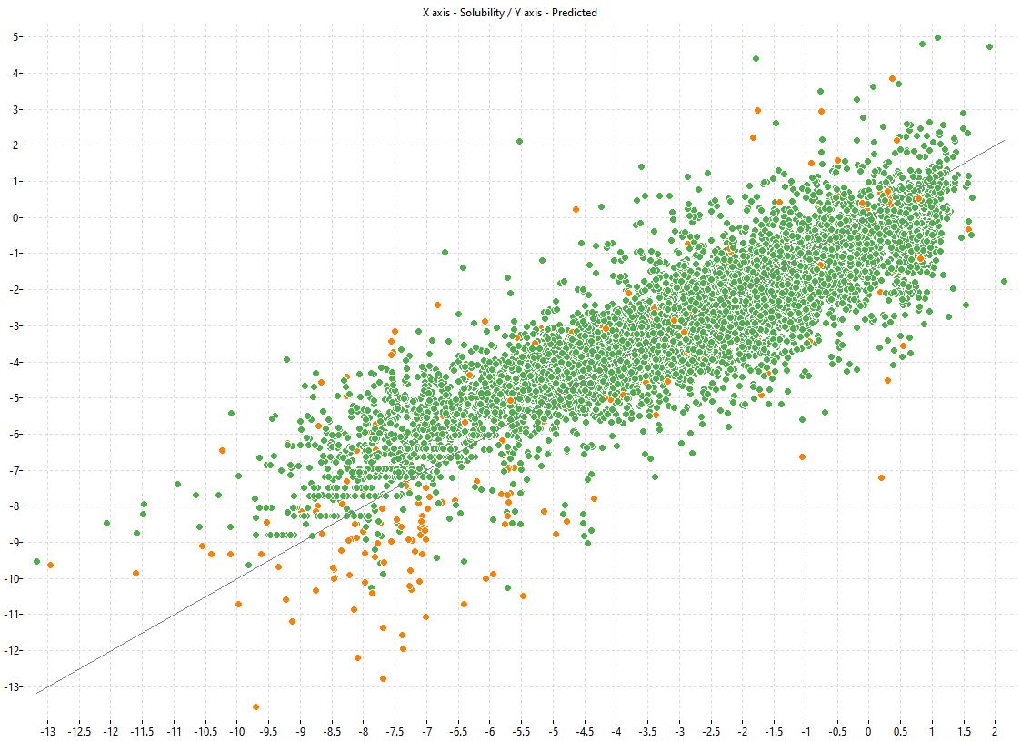 |
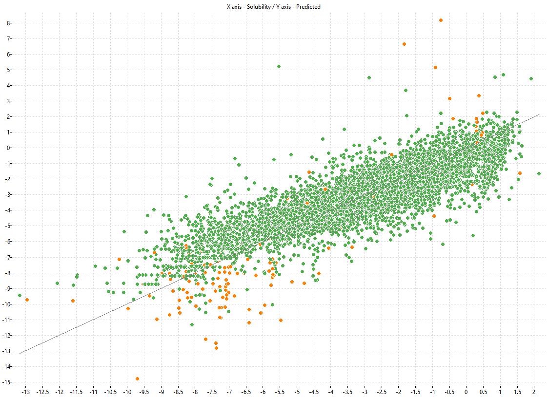 |
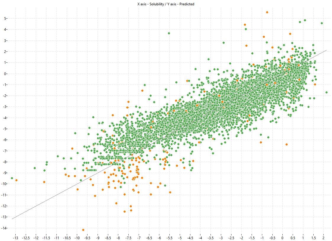 |
4. Model application and test (alvaRunner)
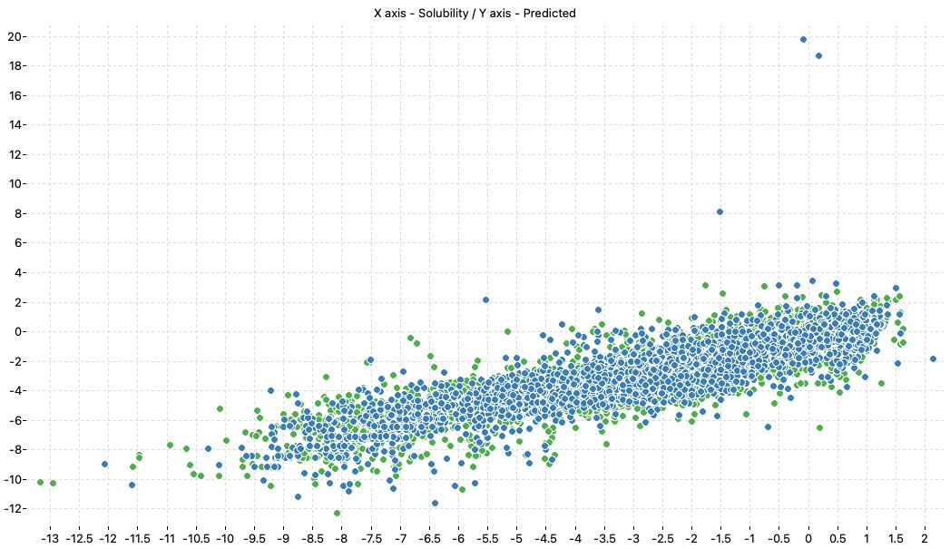
As a final step, the model selected by alvaModel have been applied on a new set of molecules using alvaRunner. Specifically, it has been applied on 1,000 chemicals randomly extracted from the metabolite structures available in the Human Metabolome Database (HMDB).
ESOL model included in alvaDesc and the models developed using alvaModel show a high correlation, as reported in the table below:
| Model name | Correlation with ESOL model |
|---|---|
| LOGS Model-1 | 0.8826 |
| LOGS Model-2 | 0.9019 |
| LOGS Consensus | 0.9027 |
